How Label Smoothing Impacts Validation Accuracy

I wrote an app to classify an object using transfer learning, and the model was trained on CIFAR-10 dataset, all by myself.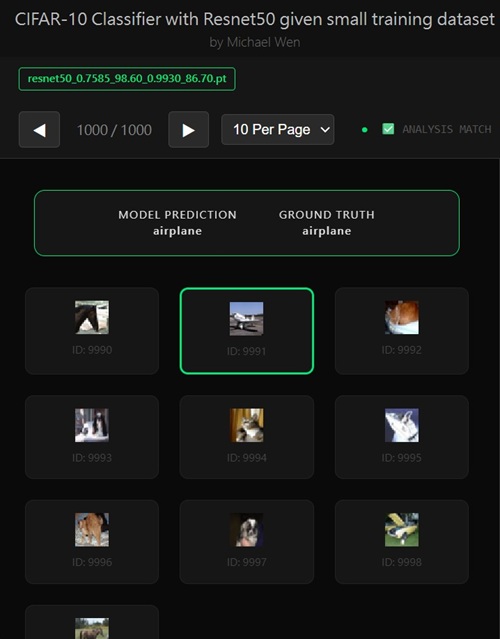

Evaluating the Effect of Label Smoothing

Motivation

To further improve validation accuracy, we explored label smoothing as an additional regularization technique. Label smoothing is commonly used in classification tasks to reduce overconfidence in neural network predictions and to improve generalization, especially when training data is limited or noisy.

How Label Smoothing Works

In standard classification, ground-truth labels are represented as one-hot vectors. For a K-class problem, the correct class is assigned probability 1.0, while all other classes receive 0.0. This hard assignment encourages the model to become extremely confident, often pushing logits to very large magnitudes.

Label smoothing relaxes this assumption by redistributing a small portion of the probability mass to non-target classes. Formally, for a smoothing factor ε:

– Target class probability becomes 1 − ε
– Each non-target class receives ε / (K − 1)

This has several important effects:
– It discourages overconfident predictions and sharp decision boundaries
– It implicitly regularizes the classifier by penalizing extreme logits
– It improves calibration, making predicted probabilities more meaningful

From an optimization perspective, label smoothing modifies the cross-entropy loss such that the model is trained to match a softer target distribution rather than a degenerate one-hot vector, which can improve stability during fine-tuning.

Concrete Example of Label Smoothing

To make label smoothing more intuitive, consider a simple example with 10 classes (as in CIFAR-10) and a smoothing factor of ε = 0.1.

Without label smoothing, a ground-truth label for class 3 would be encoded as a one-hot vector:

[0, 0, 0, 1.0, 0, 0, 0, 0, 0, 0]

With label smoothing applied, the target distribution becomes:

[0.011, 0.011, 0.011, 0.9, 0.011, 0.011, 0.011, 0.011, 0.011, 0.011]

Here, the correct class no longer carries absolute certainty. Instead, a small portion of the probability mass is distributed uniformly across the remaining classes. This forces the model to allocate some probability to alternative classes, discouraging extreme confidence and promoting smoother decision boundaries.

In practice, this subtle change helps the network focus on learning robust, discriminative features rather than simply maximizing the logit of a single class.

How Loss Is Calculated with Label Smoothing

Standard Cross-Entropy Loss (No Label Smoothing)
Assume a 3-class classification problem with ground-truth class y = 0. The true label is represented as a one-hot vector:

y = [1.0, 0.0, 0.0]

Suppose the model outputs the following predicted probabilities after softmax:

p = [0.7, 0.2, 0.1]

The cross-entropy loss is:

L = - Σᵢ yᵢ log(pᵢ) = -log(0.7) ≈ 0.357

Only the probability assigned to the correct class contributes to the loss. The model is strongly encouraged to push this value toward 1.0.

Cross-Entropy Loss with Label Smoothing
Now apply label smoothing with ε = 0.1. For K = 3 classes, the smoothed target becomes:

ŷ = [0.9, 0.05, 0.05]

Using the same predicted probabilities p, the loss becomes:

L = - (0.9 · log(0.7) + 0.05 · log(0.2) + 0.05 · log(0.1))

Numerically:

L ≈ - (0.9 · -0.357 + 0.05 · -1.609 + 0.05 · -2.303) ≈ 0.513

Unlike standard cross-entropy, all classes now contribute to the loss. The model is still rewarded for predicting the correct class, but it is also penalized for assigning near-zero probabilities to other classes.

What This Changes in Practice
– The loss no longer collapses to zero simply by making the correct class extremely confident
– Large logit gaps between classes are discouraged
– Gradients remain informative even when the model predicts the correct class with high confidence

As a result, the network learns more calibrated probability distributions and avoids overly sharp decision boundaries, which improves robustness and generalization in transfer learning scenarios.

Decision Boundaries and Logits Explained

Decision Boundaries
In a classification model, a decision boundary is the surface in feature space that separates one class from another. Intuitively, it answers the question: “At what point does the model switch its prediction from class A to class B?”

For a neural network, inputs are first mapped into a high-dimensional feature space by the backbone (e.g., ResNet). The classifier then learns boundaries in this space that partition regions corresponding to different classes. If these boundaries are too sharp, small perturbations in the input (such as noise or minor data variations) can cause large changes in prediction, leading to poor generalization.

Regularization techniques like label smoothing encourage smoother decision boundaries, meaning the model transitions more gradually between classes. This typically improves robustness to noise and unseen data.

Logits
A logit is the raw, unnormalized output of the model’s final linear layer, produced before applying the softmax function. For a K-class classifier, the network outputs K logits:

z = [z₁, z₂, ..., zₖ]

These logits represent relative evidence for each class. The softmax function converts them into probabilities:

softmax(zᵢ) = exp(zᵢ) / Σⱼ exp(zⱼ)

When a model is trained with hard one-hot labels, it is encouraged to push the correct class logit much higher than all others, often resulting in extremely large logit magnitudes. While this can reduce training loss, it also leads to overconfident predictions and brittle decision boundaries.

Label smoothing counteracts this behavior by preventing the loss function from rewarding excessively large logit gaps. As a result, logits remain better calibrated, and the model learns more stable and generalizable class separations.

Examples of Sharp vs. Smooth Decision Boundaries

Sharp Decision Boundaries
Imagine a binary image classification task that separates images into cats and dogs. Suppose the model learns a decision boundary where even a tiny change in the input can flip the prediction:

– A cat image is classified as cat with 99.9% confidence
– Adding a small amount of noise or slightly changing the lighting causes the same image to be classified as dog

This behavior indicates a sharp decision boundary. In feature space, the boundary lies extremely close to the training samples, meaning the model has tightly fit the data. While this may produce low training loss, it often results in poor generalization and high sensitivity to noise or adversarial perturbations.

Smooth Decision Boundaries
Now consider a model trained with regularization techniques such as data augmentation and label smoothing. In this case:

– A cat image is classified as cat with 85% confidence
– Small changes in pose, lighting, or background do not alter the predicted class
– The probability assigned to dog increases gradually rather than abruptly

This reflects a smooth decision boundary. In feature space, the boundary is positioned farther away from the data points, creating a margin that tolerates natural variation. Such models are more robust, better calibrated, and typically perform better on unseen data.

Why This Matters in Transfer Learning
In transfer learning, pretrained features already capture general visual patterns. Overly sharp decision boundaries in the fine-tuning stage can destroy this generalization. Encouraging smoother boundaries helps preserve the pretrained structure while allowing task-specific adaptation.

Application and Results

We integrated label smoothing into the training pipeline and reran the experiment. The observed validation accuracy increased slightly:

– Without label smoothing: 82.1%
– With label smoothing: 82.4%

At face value, this represents a modest improvement. However, given the small magnitude of the gain, it is important to interpret the result cautiously.

Why the Improvement May Be Marginal

There are several plausible reasons why label smoothing did not lead to a more substantial performance boost in this setting:

First, the model may already be well-regularized through other mechanisms such as data augmentation, partial layer freezing, and pretrained feature reuse. In such cases, the additional regularization introduced by label smoothing provides diminishing returns.

Second, label smoothing tends to be most effective when models exhibit severe overconfidence or label noise. If the dataset is relatively clean and the classifier head is not excessively overfitting, the impact of smoothing will naturally be limited.

Third, the observed improvement may fall within the variance induced by stochastic factors such as random initialization, data shuffling, and augmentation randomness. Without multiple controlled runs, it is difficult to attribute a 0.3% gain definitively to label smoothing rather than statistical noise.

Conclusion

While label smoothing produced a slight increase in validation accuracy, the effect is small and may not be statistically significant. In this project, it appears to function more as a minor stabilizer rather than a primary performance driver. As such, label smoothing remains an optional enhancement rather than a critical component of the final training configuration.

Raw Log for Your Reference

Before label smoothing is applied:

========== CONFIG ==========
NUM_CLASSES = 10
TRAINING_SAMPLE_PER_CLASS = 100
VALIDATION_SAMPLE_PER_CLASS = 100
BATCH_SIZE = 256
EPOCHS = 20
LR = 0.001
TRAINABLE_LAYERS = 2
EARLY_STOP_PATIENCE = 10
DEVICE = cuda
============================

==============================
Training model: resnet18
==============================
Epoch [01/20] Train Loss: 1.4383 | Val Loss: 2.1212 | Train Acc: 50.10% | Val Acc: 56.00%
Epoch [02/20] Train Loss: 0.4398 | Val Loss: 2.3636 | Train Acc: 85.80% | Val Acc: 59.00%
Epoch [03/20] Train Loss: 0.2316 | Val Loss: 1.4054 | Train Acc: 92.50% | Val Acc: 70.50%
Epoch [04/20] Train Loss: 0.1048 | Val Loss: 1.1404 | Train Acc: 97.50% | Val Acc: 73.50%
Epoch [05/20] Train Loss: 0.0683 | Val Loss: 0.9930 | Train Acc: 98.30% | Val Acc: 75.00%
Epoch [06/20] Train Loss: 0.0504 | Val Loss: 0.9246 | Train Acc: 99.00% | Val Acc: 76.00%
Epoch [07/20] Train Loss: 0.0265 | Val Loss: 0.8353 | Train Acc: 99.50% | Val Acc: 78.00%
Epoch [08/20] Train Loss: 0.0165 | Val Loss: 0.8222 | Train Acc: 99.80% | Val Acc: 78.10%
Epoch [09/20] Train Loss: 0.0178 | Val Loss: 0.8403 | Train Acc: 99.70% | Val Acc: 79.40%
Epoch [10/20] Train Loss: 0.0163 | Val Loss: 0.7646 | Train Acc: 99.90% | Val Acc: 80.70%
Epoch [11/20] Train Loss: 0.0093 | Val Loss: 0.7346 | Train Acc: 99.90% | Val Acc: 80.40%
Epoch [12/20] Train Loss: 0.0077 | Val Loss: 0.7318 | Train Acc: 100.00% | Val Acc: 80.50%
Epoch [13/20] Train Loss: 0.0044 | Val Loss: 0.7445 | Train Acc: 100.00% | Val Acc: 80.70%
Epoch [14/20] Train Loss: 0.0036 | Val Loss: 0.7777 | Train Acc: 100.00% | Val Acc: 79.90%
Epoch [15/20] Train Loss: 0.0104 | Val Loss: 0.7921 | Train Acc: 99.80% | Val Acc: 79.60%
Epoch [16/20] Train Loss: 0.0032 | Val Loss: 0.7568 | Train Acc: 100.00% | Val Acc: 80.00%
Epoch [17/20] Train Loss: 0.0031 | Val Loss: 0.7208 | Train Acc: 100.00% | Val Acc: 80.00%
Epoch [18/20] Train Loss: 0.0049 | Val Loss: 0.6775 | Train Acc: 99.90% | Val Acc: 80.80%
Epoch [19/20] Train Loss: 0.0033 | Val Loss: 0.6717 | Train Acc: 100.00% | Val Acc: 81.70%
Epoch [20/20] Train Loss: 0.0022 | Val Loss: 0.6731 | Train Acc: 100.00% | Val Acc: 82.10%

Best results for resnet18:
Train Loss: 0.0022 | Val Loss: 0.6731 | Train Acc: 100.00% | Val Acc: 82.10%
Training Time: 82.25 seconds

After label smoothing is applied:

========== CONFIG ==========
NUM_CLASSES = 10
TRAINING_SAMPLE_PER_CLASS = 100
VALIDATION_SAMPLE_PER_CLASS = 100
BATCH_SIZE = 256
EPOCHS = 20
LR = 0.001
TRAINABLE_LAYERS = 2
EARLY_STOP_PATIENCE = 10
DEVICE = cuda
============================

==============================
Training model: resnet18
==============================
Epoch [01/20] Train Loss: 1.6192 | Val Loss: 2.3258 | Train Acc: 51.30% | Val Acc: 61.20%
Epoch [02/20] Train Loss: 0.9005 | Val Loss: 2.0775 | Train Acc: 86.80% | Val Acc: 69.80%
Epoch [03/20] Train Loss: 0.7575 | Val Loss: 1.6626 | Train Acc: 93.70% | Val Acc: 70.70%
Epoch [04/20] Train Loss: 0.6772 | Val Loss: 1.4552 | Train Acc: 97.10% | Val Acc: 68.40%
Epoch [05/20] Train Loss: 0.6166 | Val Loss: 1.2617 | Train Acc: 99.30% | Val Acc: 71.80%
Epoch [06/20] Train Loss: 0.5969 | Val Loss: 1.1144 | Train Acc: 99.40% | Val Acc: 78.50%
Epoch [07/20] Train Loss: 0.5810 | Val Loss: 1.1111 | Train Acc: 100.00% | Val Acc: 77.10%
Epoch [08/20] Train Loss: 0.5645 | Val Loss: 1.0674 | Train Acc: 100.00% | Val Acc: 79.40%
Epoch [09/20] Train Loss: 0.5534 | Val Loss: 1.0772 | Train Acc: 100.00% | Val Acc: 79.00%
Epoch [10/20] Train Loss: 0.5458 | Val Loss: 1.0327 | Train Acc: 99.90% | Val Acc: 79.20%
Epoch [11/20] Train Loss: 0.5405 | Val Loss: 1.0147 | Train Acc: 99.80% | Val Acc: 79.60%
Epoch [12/20] Train Loss: 0.5375 | Val Loss: 0.9983 | Train Acc: 100.00% | Val Acc: 80.80%
Epoch [13/20] Train Loss: 0.5331 | Val Loss: 0.9966 | Train Acc: 99.90% | Val Acc: 81.60%
Epoch [14/20] Train Loss: 0.5282 | Val Loss: 0.9910 | Train Acc: 100.00% | Val Acc: 81.60%
Epoch [15/20] Train Loss: 0.5270 | Val Loss: 0.9795 | Train Acc: 100.00% | Val Acc: 82.40%
Epoch [16/20] Train Loss: 0.5268 | Val Loss: 0.9841 | Train Acc: 100.00% | Val Acc: 81.50%
Epoch [17/20] Train Loss: 0.5238 | Val Loss: 0.9965 | Train Acc: 100.00% | Val Acc: 81.30%
Epoch [18/20] Train Loss: 0.5231 | Val Loss: 0.9921 | Train Acc: 100.00% | Val Acc: 81.80%
Epoch [19/20] Train Loss: 0.5204 | Val Loss: 0.9781 | Train Acc: 100.00% | Val Acc: 82.20%
Epoch [20/20] Train Loss: 0.5199 | Val Loss: 0.9865 | Train Acc: 100.00% | Val Acc: 81.10%

Best results for resnet18:
Train Loss: 0.5270 | Val Loss: 0.9795 | Train Acc: 100.00% | Val Acc: 82.40%
Training Time: 102.22 seconds

Any comments? Feel free to participate below in the Facebook comment section.